Happy New Year, everyone! I have been heads-down for the past few months working on a book about enterprise Power BI projects. I have been a bit scarce online, and it’s time to come up for air and to share some things.
First, an apology to those of you who follow this blog and may have received a barrage of email notifications a while ago. When I have ideas for blog posts, I throw titles and ideas into unpublished posts and keep them in draft form so I can work on them in my spare time (which I have had little of). While sitting in a particularly interesting session as the PASS Data Community Summit in early November, I went to add another idea, but my laptop was dead, so I opened the WordPress app on my phone and proceeded to accidentally publish every empty post in my Drafts folder, which send 13 email messages to 7,000 people. It was a senior moment. If you want to know what I will be posting in the next couple of months, go check your inbox on Nov 7th :-).
I wanted to share the results of a few experiments I recent conducted with one of my favorite sets of sample data. This will take at least two blog posts to cover, but I will summarize them here:
- Compare data load & transformations with CSV files vs a Fabric lakehouse using the SQL Server connector:
Loading 20 million fact rows from CSV files vs a Fabric lakehouse, using Power Query.
Same comparison with deployed Power BI model. - Comparing Fabric data transformation options & performance:
Loading & transforming the same data with Power BI Desktop, Fabric Gen2 dataflows, Fabric pipelines and Spark notebooks. - Comparing semantic model performance in Fabric and Power BI:
Report & semantic model performance comparing the same data in Import mode, DirectQuery and Direct Lake.
Experiment #1:
Compare loading & transforming data from CSV files vs a Fabric lakehouse using the SQL Server connector
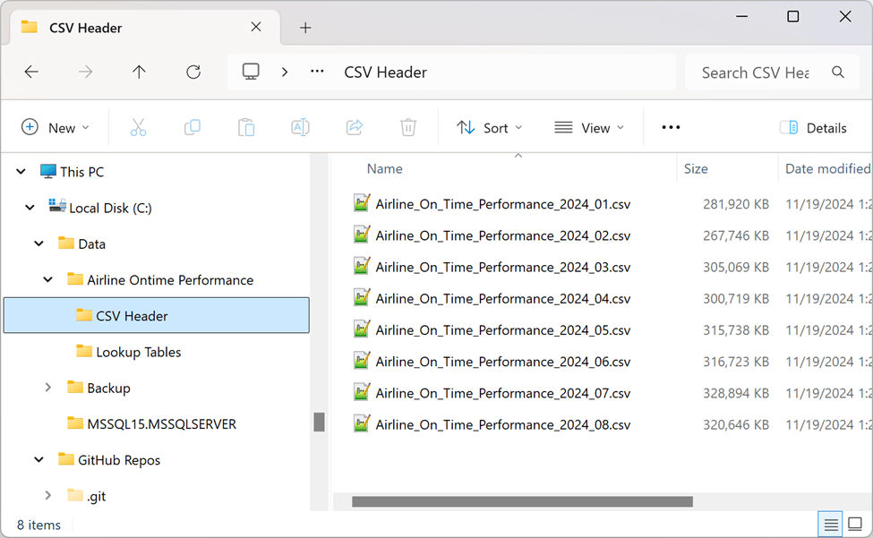
I’ve downloaded 32 months of airline performance data from the US Department of Transportation. The data source is a set of files containing flight records for every commercial airline flight between mid-size and large US airports. This is real data that any traveler should understand and appreciate. If you have heard an airline claim to be ranked highly in on-time performance compared to their competitors, those statistics, come from this data.
The United States Department of Transportation (USDOT) publishes detailed airline and flight performance information through a department called the Bureau of Transportation Statistics (BTS). Monthly data files can be downloaded from the BTS site containing flight records up to a few months prior to the current date. Files contain one record per flight with about 500,000 to 800,000 flights per month. Each monthly file ranges in size, about 250 to 350 megabytes each.
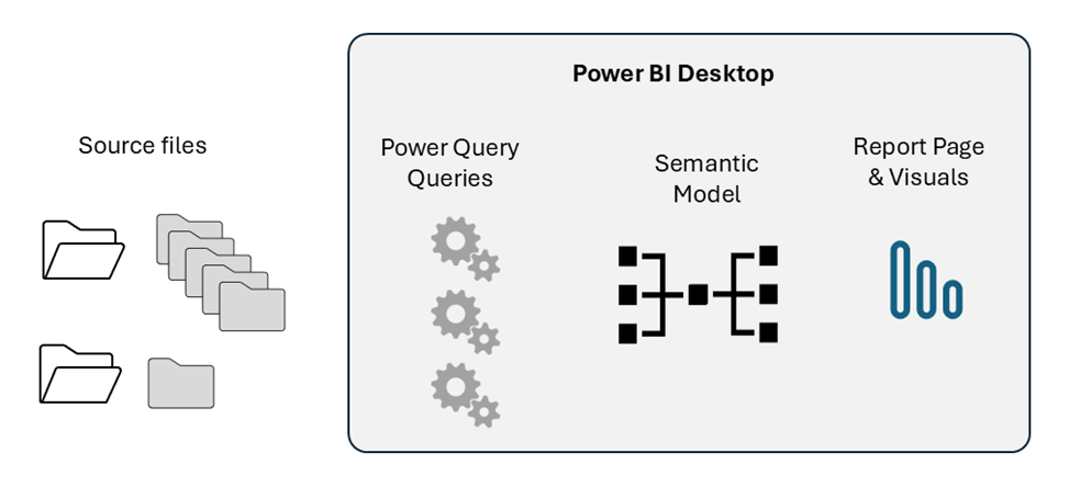
Each flight record contains the airline code, flight number, aircraft tail number, origin and destination airport information, and event times including the scheduled departure time, actual departure time, wheels-off time, wheels-on time, scheduled arrival time and actual arrival time, and some assorted durations and category fields. The architecture of this first project is pretty simple. Using Power Query in Power BI Desktop, files are imported from CSV files stored in local folders. Once deployed to the service the same files could either be accessed through an on-premises gateway or the files could be moved to an Azure BLOB container to be accessed online.
To start, I’ll import only the 8 months of data that is available for 2024 so far (it takes the DOT a few months to make the data available for download). The plan is to add monthly files for multiple previous years later on.
Importing the contents of this folder causes Power Query to generate a function and parameter that it uses to import and merge into a single table within the query. If you have imported the contents of a folder in Power Query, you’ve probably seen how this works.
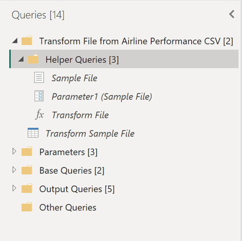
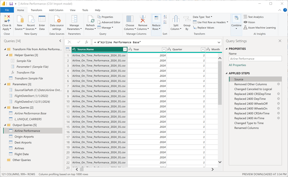
After performing so data cleanse, I saved this query and disabled data load so it can be used to build multiple tables in the dimensional model. I’ve called this query Airline Performance Base because it will be used as the base reference query to load the Airlines, Origin Airports and Destination Airports tables, in addition to the Airline Performance fact table containing all the flight details and performance metrics.
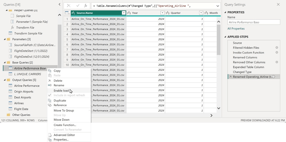
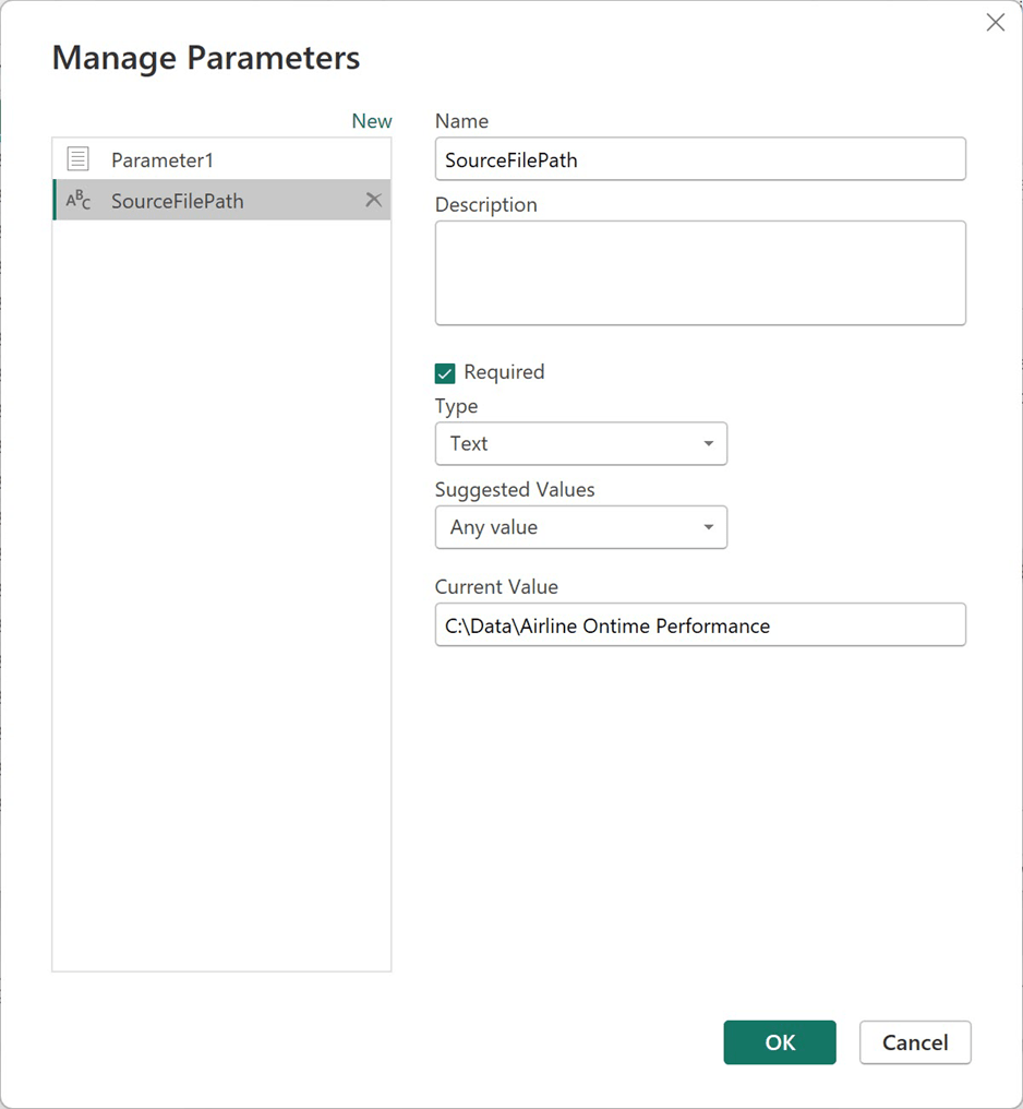
I always use parameters to manage things like source file paths, server name, database name, and date ranges for filtering fact tables. My source files are in a subfolder under this folder. the path is managed in the SourceFilePath parameter.
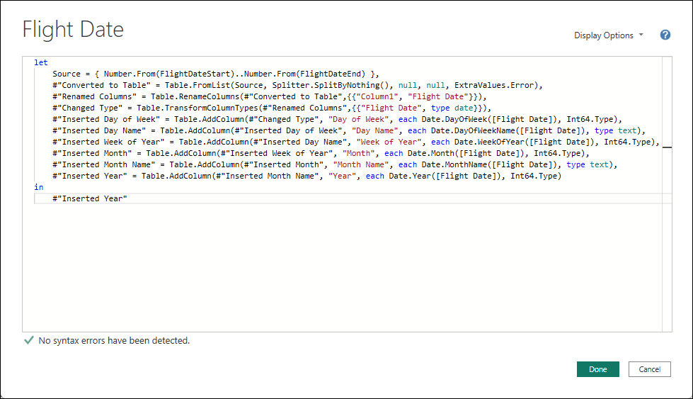
The Airlines query merges the contents of a CSV files containing 700 airline carrier names with the airline codes in the Airline Performance Base query. This is so we only include the 30 major airlines we care about for reporting. The Origin Airports and Dest Airports queries are derived directly from columns in the Airline Performance Base query. Rows are deduplicated and cleaned-up. The Flight Date dimension table is generated in Power Query using this M script:
The Airline Performance query will populate the main fact table. One interesting problem with this set of data is that the six time-value columns, store a four-digit number as text in the CSV files, use “2400” to represent midnight. That value causes an error because we database people consider midnight to be the first, rather than last minute of the day, or “0000”. The US Navy started recording time that way about 105 years ago, and the standard was then adopted by the aviation industry. After making this correction, all the four-digit values will convert correctly to the Time data type.
For brevity, there are a lot of details that I will cover in the book, that I am abbreviating here so we can get to the results of the experiment.
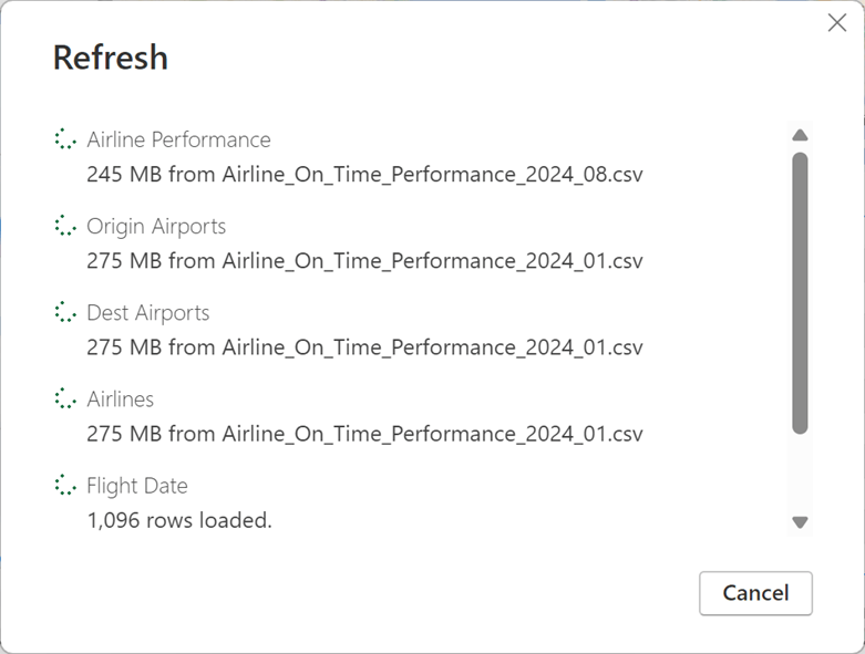
It took about six minutes to process eight months of data on my machine. That’s about 45 seconds per file – not too shabby. Then I add the monthly files for 32 months of source data and see what happens.
With all files in the source folder, I click the Refresh button on the Home ribbon and…
It took 30 minutes to load 32 monthly files, containing about 20 million rows of data.
There are a few variables in this experiment that should be taken into consideration. One factor is that the file size isn’t the same every month and these file sizes tend to increase a little over time as the airlines add more flights. But, by doing some rough math, we can see that the time per file increases a little as more files are added. Loading nearly three years of data is manageable. But what about five years or ten years of data?
In the current solution, we add new records by dropping new files into the source folder and then refresh the entire dataset. Since the historical data doesn’t change, the same old data will have to be reprocessed every time we need to refresh the semantic model.
Importing Data from a Database
If the same data were imported from a relational database or managed data source capable of running SQL queries, that should simplify the process for getting data into the semantic model. The following example uses the SQL Server connector which will work with the same data stored in an on-premises SQL Server database, an Azure SQL database, a Fabric lakehouse or warehouse. Power BI wouldn’t even know the difference and would just work.
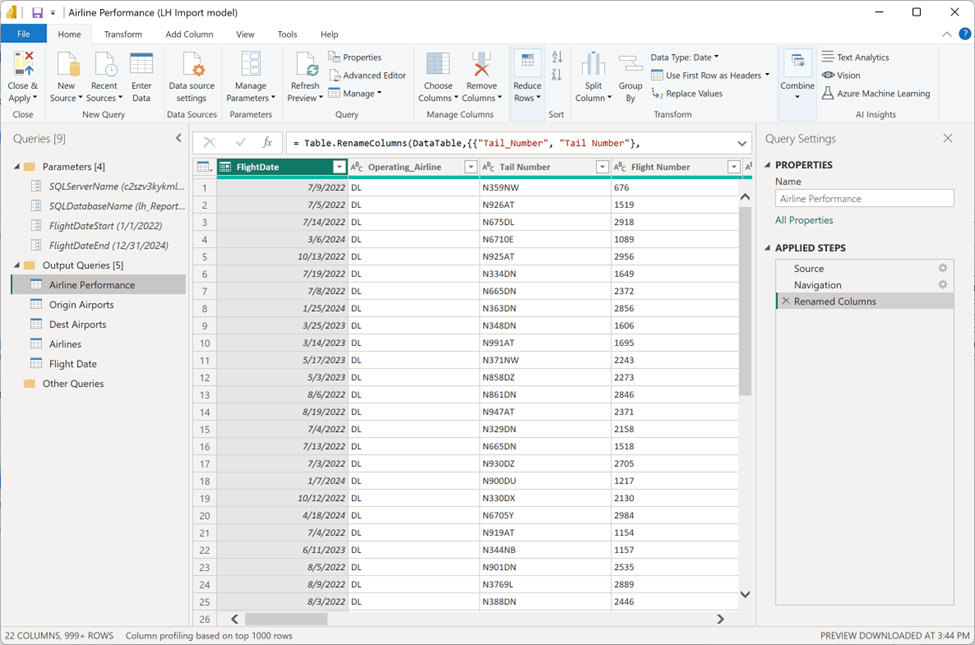
Back in Power BI Desktop, my modified Power Query solution with all the queries connected to a Fabric lakehouse using SQL Server connections. Each query is considerably simple compared to the previous exercise because most of the transformations occurred before loading the lakehouse tables. The only caveat is that, unlike SQL Server or a Fabric warehouse, a Fabric lakehouse doesn’t support table or column names containing spaces, so I have a step that renames the columns.
Like the file-based queries, I use parameters to store the server name (actually the lakehouse SQL endpoint) and the database name (which is the lakehouse name when using the SQL endpoint).
By comparison, the data refresh goes pretty quickly.
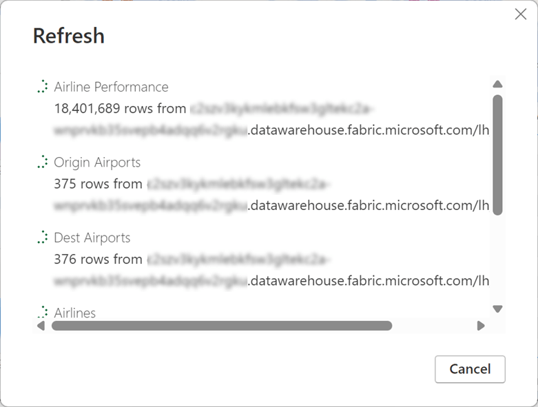
It took only six minutes to load all 20 million rows of data.
So far, I was able to reduce the load time by a factor of five by moving the data source from CSV files to a SQL database (a Fabric lakehouse with the SQL endpoint in this case).
What other optimizations can be made? Since the data source supports efficient query folding and historical data remains static, let’s use Incremental refresh to partition the fact table and only load new records rather than reloading the whole thing every time a Refresh is performed.
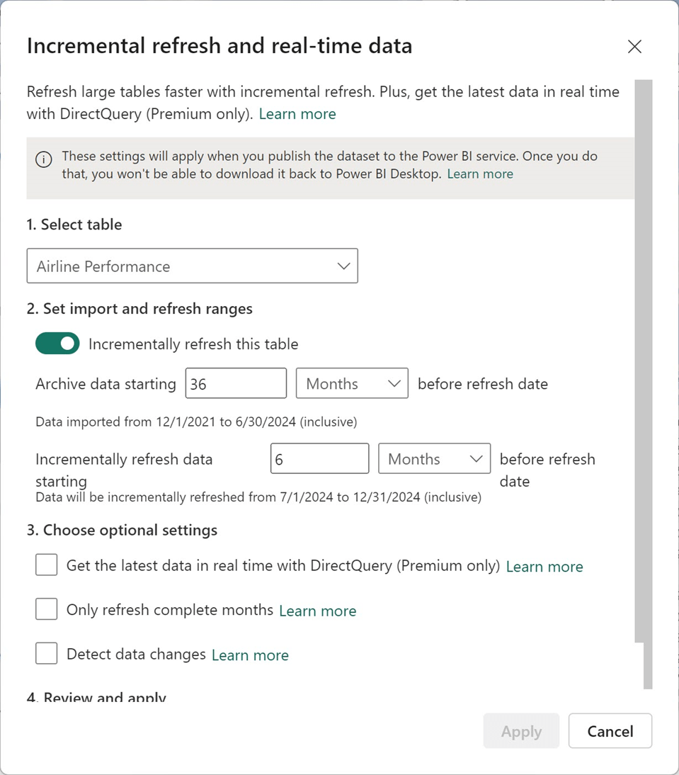
I set up Incremental refresh using RangeStart and RangeEnd parameters. I use these parameters to filter a date/time type column in the Airline Performance table.

…then configure Incremental refresh to partition up to 3.5 years of data using monthly partitions.
I deployed the semantic model and report to the service, setup connection credentials, and then refreshed the model. With the semantic model and lakehouse in the same workspace (and therefore, the same capacity and region), the initial refresh time was only three minutes. During that time, it created and processed 32 separate partitions.
Running a subsequent refresh took less than a minute. No data was actually processed because all the historical data had already been loaded into the model. In theory, if new records had been added within the past six months, that could have added a few more seconds to the run time. Regardless, this is very fast compared to the initial load and query times.
Performance Results
Here are the results of the experiment using the same volume of data for each scenario:
| Scenario | Data refresh time |
| Power Query loading from local CSV files | 30 minutes |
| Power Query loading from lakehouse with SQL endpoint | 6 minutes |
| Incremental refresh – Initial load and processing | 3 minutes |
| Incremental refresh – Subsequent processing | 1 minute |
An important point is that if the source data were in fact a set of monthly CSV files that would need to be loaded into the lakehouse or SQL database, aren’t we really just moving that part of the process upstream to the ETL process, prior to the data store used by Power Query? Yes, that is true but there are other advantages to compartmentaizing the data engineering effort. That part of the experiment will be covered in a follow-up post. To tee that up, here is the architecture for the modified solution using Microsoft Fabric, that I will explain in the next post. I will move the Power Query queries from Power BI Desktop into Gen2 Dataflows in a Fabric workspace so we can compare the performance and possible advantages to moving them. I will also perform the same transformation logic using other Fabric ETL components like pipelines and Spark notebooks.
Stay tuned. Thanks for reading.


neat! Sources Suggest [Potential Collaboration] on [Scientific Research] 2025 great